Using the geocode Parameter for Spatial Analysis

library(susR)      
library(dplyr)
#> 
#> Attaching package: 'dplyr'
#> The following objects are masked from 'package:stats':
#> 
#>     filter, lag
#> The following objects are masked from 'package:base':
#> 
#>     intersect, setdiff, setequal, union
library(ggplot2)
library(stringr)
library(tidyr)
library(purrr)
library(sf)
#> Linking to GEOS 3.12.1, GDAL 3.8.4, PROJ 9.4.0; sf_use_s2() is TRUE

Introduction

In this vignette, we demonstrate how to use the new geocode functionality in the susR package, specifically in fetch_susr_data() function. This feature adds geometry to the results of an API call, allowing users to create spatial visualizations directly from the dataset.

Additionally, we can now use “wrappers” for regional selection, including districts, NUTS2, NUTS3, country, lau1, and more. These wrappers simplify selecting different levels of administrative regions, making spatial analysis more flexible.

params_districts <- list(
  "om7005rr", # table code
  list(
    "Districts", # vector of district codes 
    c(1996, 2023),           # years
    "IN010089",              # mean age
    "SPOLU"                  # sex: SPOLU = Total
    )
)

params_NUTS3 <- list(
  "om7005rr", # table code
  list(
    "NUTS3", # vector of district codes 
    c(1996, 2023),           # years
    "IN010089",              # mean age
    "SPOLU"                  # sex: SPOLU = Total
    )
)

Districts data

We first fetch the data for districts, utilizing the geocode parameter to include spatial information.

res <- fetch_susr_data(params_districts, geocode = TRUE)

cleaned_age_df <- res[["om7005rr"]] |> 
  rename( # renaming to more user-friendly names
    district = om7005rr_vuc,
    year  = om7005rr_obd,
    mean_age  = value,
    sex = om7005rr_poh
  ) |> 
  select(district, year, sex, mean_age, geometry) |> 
  pivot_wider(values_from = mean_age,
              names_from = year) |> 
  mutate(diff = `2023` - `1996`) |> 
  select(-`1996`,
         -`2023`,
         -sex) |> 
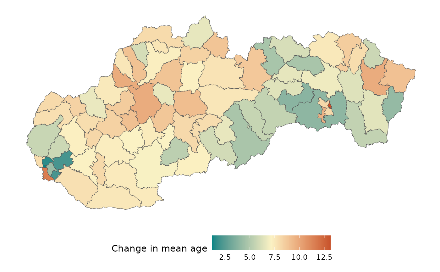
  st_as_sf()

Visualization of District-Level Data

The following map illustrates the change in mean age across districts over the selected years.

midp <- mean(cleaned_age_df$diff)

cleaned_age_df |> 
  ggplot() +
  geom_sf(mapping = aes(fill = diff)) +
  scale_fill_gradient2(name = "Change in mean age",
                       low = "#008585",
                       mid = "#fbf2c4",
                       high = "#c7522b",
                       midpoint = midp) +
  theme_minimal() +
  theme(
    panel.grid.major = element_blank(),
    axis.text = element_blank(),
    legend.position = "bottom",
    legend.key.width = unit(1, 'cm')
  )

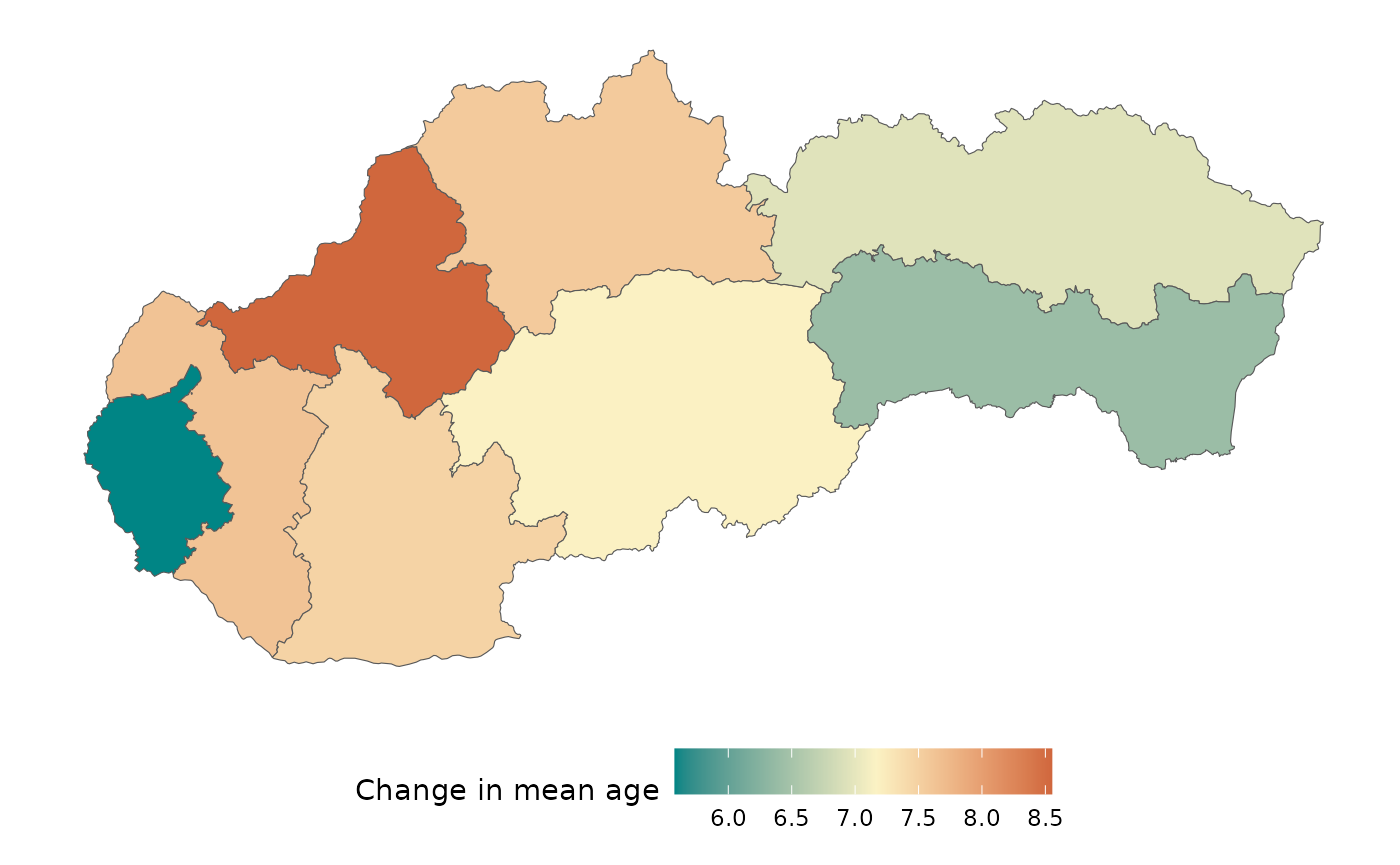
NUTS3 data

We repeat the process for a higher regional level (NUTS3).

res <- fetch_susr_data(params_NUTS3, geocode = TRUE)

cleaned_age_df <- res[["om7005rr"]] |> 
  rename( # renaming to more user-friendly names
    region = om7005rr_vuc,
    year  = om7005rr_obd,
    mean_age  = value,
    sex = om7005rr_poh
  ) |> 
  select(region, year, sex, mean_age, geometry) |> 
  pivot_wider(values_from = mean_age,
              names_from = year) |> 
  mutate(diff = `2023` - `1996`) |> 
  select(-`1996`,
         -`2023`,
         -sex) |> 
  st_as_sf()

Visualization of NUTS3-Level Data

Similarly, the following map displays the change in mean age at the NUTS3 level.

midp <- mean(cleaned_age_df$diff)

cleaned_age_df |> 
  ggplot() +
  geom_sf(mapping = aes(fill = diff)) +
  scale_fill_gradient2(name = "Change in mean age",
                       low = "#008585",
                       mid = "#fbf2c4",
                       high = "#c7522b",
                       midpoint = midp) +
  theme_minimal() +
  theme(
    panel.grid.major = element_blank(),
    axis.text = element_blank(),
    legend.position = "bottom",
    legend.key.width = unit(1, 'cm')
  )

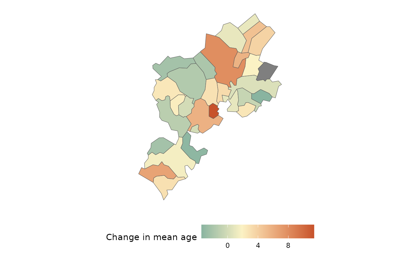
Municipalities data

We now perform the same process for the smallest available regional level—municipalities. Due to the high granularity, we recommend filtering the dataset to include only relevant records for your analysis. This method is not (yet) optimized for handling a large volume records.

If you require data for all municipalities in Slovakia, consider using the giscoR package with the gisco_get_communes() or gisco_get_lau() functions. These functions allow you to retrieve geospatial data, which you can then manually join with the results from fetch_susr_data().

mun_res <- susr_dimension_values("om7052rr",
                             "om7052rr_obc") |> 
  filter(str_detect(element_value, "SK0108")) |> 
  mutate(code = substr(element_value, nchar(element_value) - 5, nchar(element_value)))

params_mun <- list(
  "om7052rr", # table code
  list(
    mun_res$element_value, # vector of district codes 
    c(1996, 2023),           # years
    "IN010089",              # mean age
    "SPOLU"                  # sex: Spolu = Total
    )
)

res <- fetch_susr_data(params_mun, geocode = TRUE)

cleaned_age_df <- res[["om7052rr"]] |> 
  filter(code %in% mun_res$code) |> 
  rename( # renaming to more user-friendly names
    region = om7052rr_obc,
    year  = om7052rr_obd,
    mean_age  = value,
    sex = om7052rr_poh
  ) |> 
  select(region, year, sex, mean_age, geometry) |> 
  pivot_wider(values_from = mean_age,
              names_from = year) |> 
  mutate(diff = `2023` - `1996`) |> 
  select(-`1996`,
         -`2023`,
         -sex)|> 
  st_as_sf()

Visualization of NUTS3-Level Data

Similarly, the following map displays the change in mean age at the NUTS3 level.

midp <- mean(cleaned_age_df$diff, na.rm = TRUE)

cleaned_age_df |> 
  ggplot() +
  geom_sf(mapping = aes(fill = diff)) +
  scale_fill_gradient2(name = "Change in mean age",
                       low = "#008585",
                       mid = "#fbf2c4",
                       high = "#c7522b",
                       midpoint = midp) +
  theme_minimal() +
  theme(
    panel.grid.major = element_blank(),
    axis.text = element_blank(),
    legend.position = "bottom",
    legend.key.width = unit(1, 'cm')
  )

Conclusion

The geocode parameter in fetch_susr_data() enables users to retrieve spatial information and create insightful maps. This functionality is valuable for analyzing regional trends and making data-driven decisions based on spatial patterns.